Simulating Phylogenetically Structured Networks*

*Contributed by Vinicius Bastazini and Vanderlei Debastiani

“Nothing in biology makes sense except in the light of evolution.” (Dobzhansky 1973)

“Nothing in evolutionary biology makes sense except in the light of ecology.” (Grant and Grant 2008)

“Nothing in evolution or ecology makes sense except in the light of the other. ” (Pelletier et al. 2009)

Understanding the interplay between evolutionary and ecological processes is crucial for describing patterns of species diversity in space and time. Historically, community ecology and evolutionary biology have followed separate paths. However, in the past decades, the inclusion of phylogenetic data has expanded the toolkit for community ecologists, shedding light on large range of biological processes such as species interactions, community assembly and disassembly, species distribution, and ecosystem functioning. Phylogenetic information has also provided a sort of  “temporary” solution for missing data in ecological databases.

This novel and integrative approach has given rise to Ecophylogenetics, an interdisciplinary field of study that combines principles from both ecology and phylogenetics. It focuses on understanding the evolutionary relationships among species in the context of ecological processes and patterns. 

In this context, phylogenetically structured models have thus revolutionized our understanding of ecological phenomena, by providing a framework to explore and interpret the patterns of species evolution, diversity, and interactions. This is especially relevant in Network Ecology, a branch of ecology interested in investigating the structure, function, and evolution of ecological systems using network models and analyses. Phylogenetic approaches have been incorporated into the study of ecological networks formed by interacting species, in order to describe distinct ecological phenomena, such as network assembly and disassembly (see a related post here),  and its ability to cope with cascading effects such as species loss (see a related post here). 

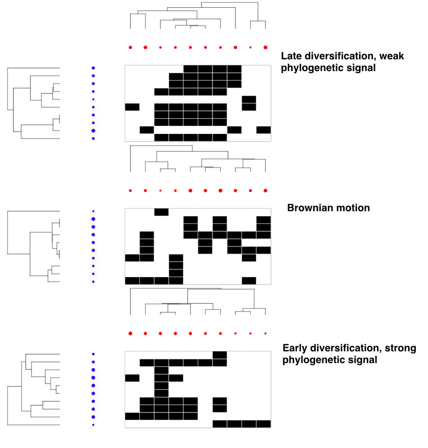
Examples of some of the possible eco-evolutionary dynamics of bipartite mutualistic networks. Species interactions are represented by black cells in the bi-adjacency matrices along with their evolutionary trees and traits ( blue and red circles). Trait values are represented by circle size.

In the following example, we will demonstrate how to simulate phylogenetically structured networks using  R.

In this example we will simulate ultrametric phylogenetic trees for two distinct sets of species, such as consumers ( e.g., predator, pollinator or seed disperser) and resources (prey, flowering plants), following a uniform birth–death process, which reflects the underlying evolutionary dynamics of taxa. Additionally, we will simulate the evolution of a single trait by employing a family of power transformations to the branch lengths of these simulated phylogenetic trees. The choice of this transformation parameter defines the tempo and mode of trait evolution. Networks of interacting species will be generated using a single-trait complementarity model (Santamaria and Rodriguez-Girones 2007). According to the single-trait complementarity model, each species in the network is represented by a mean trait value and its variability, and a pair of species is more likely to interact if their trait values overlap. You can find further information on this sort of simulation  in Debastiani et al. (2021a, 2021 b) and Bastazini et al. (2022).

#### Load R packages
require(ape)
require(geiger)
require(plotrix)

#### Define phylo_web, a function  that generates phylogenetic structured networks
# The inputs are: number of species in each set of interacting species and the level of phylogenetic signal

phylo_web = function(n_spe_H, n_spe_L, power_H, power_L) {
  
  # Generate a phylogenetic tree for consumer species (H)
  tree_H = geiger::sim.bdtree(b = 0.1, d = 0, stop = "taxa", n = n_spe_H, extinct = FALSE)
  for (y in 1:length(tree_H$edge.length)) {
    if (tree_H$edge.length[y] <= 0)
      tree_H$edge.length[y] = 0.01
  }
  
  # Generate a phylogenetic tree for resource species  (L)
  tree_L = geiger::sim.bdtree(b = 0.1, d = 0, stop = "taxa", n = n_spe_L, extinct = FALSE)
  for (y in 1: length(tree_L$edge.length)) {
    if (tree_L$edge.length[y] <= 0)
      tree_L$edge.length[y] = 0.01
  }
  
  # Assign labels to the tips of the trees
  tree_H$tip.label = sprintf("H_%.3d", 1:length(tree_H$tip.label))
  tree_L$tip.label = sprintf("L_%.3d", 1:length(tree_L$tip.label))
  
  # Generate trait data for consumers
  trait_H = matrix(NA, nrow = n_spe_H, ncol = 1)
  for(n in 1:1) {
    trait_H[, n] = ape::rTraitCont(compute.brlen(tree_H, power = power_H), model = "BM")
  }
  trait_H[,1] = plotrix::rescale(trait_H[,1], newrange = c(0, 1))
  rownames(trait_H) = tree_H$tip.label
  colnames(trait_H) = sprintf("Tr_H_%.3d", 1:ncol(trait_H))
  
  # Generate trait data for resources
  trait_L = matrix(NA, nrow = n_spe_L, ncol = 1)
  for(n in 1:1) {
    trait_L[, n] = ape::rTraitCont(compute.brlen(tree_L, power = power_L), model = "BM")
  }
  trait_L[,1] = plotrix::rescale(trait_L[,1], newrange = c(0, 1))
  rownames(trait_L) = tree_L$tip.label
  colnames(trait_L) = sprintf("Tr_L_%.3d", 1:ncol(trait_L))
  
  # Generate bi-adjacency interaction  matrix based on trait differences and niche overlap
  d_H = matrix(runif(n_spe_H, max = 0.25), nrow = n_spe_H, ncol = 1)
  d_L = matrix(runif(n_spe_L, max = 0.25), nrow = n_spe_L, ncol = 1)
  web = matrix(NA, nrow = n_spe_L, ncol = n_spe_H)
  for(i in 1:n_spe_L) {
    for(j in 1:n_spe_H) {
      II = abs(trait_H[j] - trait_L[i])
      III = 0.5 * (d_H[j] + d_L[i])
      web[i,j] = ifelse(II < III, yes = 1, no = 0)
    }
  }
  colnames(web) = tree_H$tip.label
  rownames(web) = tree_L$tip.label
  
  # Ensure there are no species with no interactions
  z_H = which(colSums(web) == 0)
  if (length(z_H) > 0) {
    for(i in 1:length(z_H)) {
      web[sample(1:n_spe_L, size = 1), z_H[i]] = 1
    }
  }
  z_L = which(rowSums(web) == 0)
  if (length(z_L) > 0) {
    for(i in 1:length(z_L)) {
      web[z_L[i], sample(1:n_spe_H, size = 1)] = 1
    }
  }
  
  # Return the results as a list
  RES = list(tree_H = tree_H, tree_L = tree_L, trait_H = trait_H, trait_L = trait_L, web = web)
  return(RES)
}

#### Generate networks  using the phylo_web function

# Here, we are  generating a network formed by 10 resource species (e.g., flowers) , 10 consumers (pollinators),  simulating a Brownian motion process for trait evolution:

n_spe_HA = 10 # Number of consumer species 
n_spe_LA = 10 # Number of resource species 
power_HA = 1 # Grafen's rho of consumer species
power_LA = 1  # Grafen's rho of resource species

web = phylo_web(n_spe_HA, n_spe_LA, power_HA, power_LA)

# The result is list containing  a bi-adjacency matrix for two sets of interacting species,  their phylogenies and trait values.

web

Now we can plot the bi-adjacency matrix along with their evolutionary trees and traits. Trait values are represented by circle size.

# Create and arrange the plot for the phylogenetic trees, species traits, and the network

par(mar = c(0.4, 0.4, 0.4, 0.4))
layout(matrix(c(0, 0, 1, 0, 0, 2, 3, 4, 5), nrow = 3, ncol = 3, byrow = TRUE), 
       widths = c(0.4, 0.4, 1), 
       heights = c(0.4, 0.4, 1))


# Plot
ape::plot.phylo(web$tree_H, show.tip.label = FALSE, 
     direction = "downwards")
plot(web$trait_H[,1], rep(1, times = length(web$trait_H[,1])), 
     xlab = "", ylab = "", 
     xaxt = "n", yaxt = "n", 
     type = "n", bty = "n",
     ylim = c(0.9, 1.1), xlim = c(1, length(web$trait_H[,1])))
points(1:length(web$trait_H[,1]), rep(1, times = length(web$trait_H[,1])),
       cex = web$trait_H[,1]+1, pch = 19)
ape::plot.phylo(web$tree_L, show.tip.label = FALSE,
     direction = "rightwards")
plot(web$trait_L[,1], rep(1, times = length(web$trait_L[,1])),
     xlab = "", ylab = "", 
     xaxt = "n", yaxt = "n", 
     type = "n", bty = "n",
     xlim = c(0.9,1.1), ylim = c(1, length(web$trait_L[,1])))
points(rep(1, times = length(web$trait_L[,1])), 1:length(web$trait_L[,1]),
       cex = web$trait_L[,1]+1, pch = 19)
plotrix::color2D.matplot(web$web,
                cs1 = c(1, 0), cs2 = c(1, 0), cs3 = c(1, 0), 
                yrev = FALSE,
                ylab = "", xlab = "", 
                xaxt = "n", yaxt = "n",
                border="white", axes = FALSE)

Et voilà!!!

Evolution drives the ability of mutualistic networks to cope with trait-based co-extinction cascades

The fast pace of the current anthropogenic-induced mass extinction has demanded conservation scientists to ​provide high-quality information that can guide policies aiming to minimize and mitigate the impacts of biodiversity loss. As no species lives alone in the environment, understanding how species loss can cascade across ecosystems through the networks formed by organisms and their interactions has become a major challenge. Empirical evidence shows that the loss of a single species may create a domino effect, resulting in the extinction of other species or even entire ecosystems. These cascading effects might be even more pervasive and severe in some ecological systems such as mutualisms, in which species exploit each other for mutual net benefits (Dunn et al. 2009). Ecologists believe that nearly every species is involved in at least one mutualistic interaction (Bronstein 2015). Consequently, this ubiquitous type of ecological interaction has important ecological and evolutionary implications for the maintenance of ecosystem diversity, functioning and stability.

Another complicating factor in studying cascading effects in ecological communities, is that organisms come in a complex array of forms, behaviors and functions, a dimension of biodiversity known as Functional diversity. It implies that the role an organism plays in an ecosystem is not determined by its taxonomic identity, but rather by its behavioral and morphological traits. Although every species differs from one another, they are not equally different, and some species may have disproportionate effects on ecosystems due to their unique set of traits. In an earlier contribution, we have shown that the loss of functional distinctiveness – a facet of functional diversity that warrants unique ecological interactions – takes a larger toll in ecological communities than the loss of taxonomic units alone. As species traits are largely a legacy of their evolutionary history, we might expect that the mode and tempo of trait evolution may play an important role in ecological dynamics and how ecological communities respond to perturbations. For instance, ecological communities in which species interactions have a strong phylogenetic component are more likely to suffer co-extinctions following primary extinction events (Rezende et al. 2007). 

In a recent paper, we evaluated how evolutionary dynamics affects trait-based cascades in theoretical mutualistic communities, using minimal model systems of phylogenetically structured mutualistic networks. To do so, we simulated the evolutionary dynamics of bipartite mutualistic networks, formed by two sets of interacting species, in which species interactions are generated by a single-trait complementarity model. This modeling approach mimics ecological networks such as a pollination network formed by flowering plants and birds, in which species interactions is determined by flowers’ corolla length and birds’ bill length. Traits were simulated under distinct evolutionary dynamics:

• Traits following a random walk through evolutionary time (i.e., Brownian motion model of trait evolution);

• Recent diversification of traits with low phylogenetic signal (i.e., the tendency of related species to resemble each other more than species drawn at random from the same tree);

• Early diversification of traits with a strong phylogenetic signal.

We explored the effects of primary extinctions based on two specific dimensions of functional diversity expected to have strong consequences to ecological dynamics: size-related traits (a proxy of body size) and trait distinctiveness. We then estimated  network robustness, a measure of the tolerance of a network to species loss based on ‘knockout extinction simulations’. The main idea behind robustness analyses is to evaluate co-extinction rates and their impacts on the integrity of a network (For more details in this kind of analysis see a post Frederico has recently written, and , a post I have written for a related paper here). In our case, we simulated three scenarios of primary species loss :

• Random extinctions, which serves as a baseline scenario;
• Loss of functional distinctiveness, in which species that are more different to the others in terms of their trait values are sequentially eliminated;
• Extinctions biased towards larger sizes, in which species with larger trait values are eliminated first.

Examples of some of the possible eco-evolutionary dynamics of bipartite mutualistic networks we adopted in our paper. Species interactions are represented by black cells in the bi-adjacency matrices along with their evolutionary trees and traits ( blue and red circles). Trait values are represented by circle size.

In a nutshell, the results of our simulations suggest that mutualistic networks are especially vulnerable to extinctions based on trait distinctiveness, more so than size-based extinctions. This is an important result because it reinforces the notion that the role that functionally unique species perform in ecological systems, cannot be compensated for by the remaining species. Functionally distinct species are irreplaceable components of ecosystems, and yet, this facet of functional diversity still ignored in most conservation practices. This result stress a need to refocus conservation agenda towards species that play unique roles in ecosystems.

We also show that the mode of trait evolution affects how networks cope with trait-based cascades and that co-extinction cascades spread across phylogenetically related species, increasing the erosion of biodiversity. Networks in which phylogenetic signal in traits are strong are less robust than networks with weak phylogenetic signal, which means that mutualistic networks based upon current adaptations are more likely to cope with extinction dynamics than networks that are based upon conserved traits.

Despite its simplicity, our modeling  approach reveals the importance of taking evolutionary dynamics into account in order to describe and predict the effects of extinctions cascades in ecological systems. To find out more, read our new paper “The role of evolutionary modes for trait-based cascades in mutualistic networks” just published in the journal Ecological Modelling.

Darwin to the Rescue: Using Phylogenetic Information to Overcome the Raunkiaeran Shortfall

Functional trait-based research has a unifying role in ecology, allowing the integration of ecological and evolutionary dynamics across different levels of biological organization and across spatial-temporal scales. The basic rationale underlining functional ecological studies relies on the fact that the role a organism play in an ecosystem is not determined by its taxonomic identity, but rather by its behavioral and ecological characteristics, which can differ within and between species. Thus, functional trait research offers complementary views to the classic taxonomic approach, providing a crucial step forward to reveal mechanisms driving biotic interactions and patterns of community assembly and disassembly, and ecosystem functioning.

Despite its promising role in ecology, trait-based research still very limited by data availability. This limitation is now recognized as one of the most important shortfalls hindering scientific progress in the fields of ecology and evolutionary biology, the so-called Raunkiaeran shortfall. Sampling species traits is both time consuming and expensive . Thus, data imputation has become an inherent part of data processing and analysis in functional ecology. The ecologist’s tool kit of data imputation techniques is quite broad, and encompasses a wide range of statistical techniques, from simply imputing missing values based on average trait values to more elegant statistical tools based on machine learning. Among these procedures, the use of random forests based on phylogenetic information has been a promising one. 

Just as with functional ecology, the limitation of our knowledge of the phylogenetic relationship among all living species, aka the Darwinian Shortfall also imposes another great restrain of our understanding of biodiversity. However, over the past decades, ecologists have witnessed a rapid rise in the availability of extensive phylogenies of some of the most important taxonomic groups. Although we are also far from resolving the Darwinian Shortfall, this progress in phylogenetics has proved to be a powerful tool to impute missing data in trait databases until more refined information is collected.

In our recent paper “Using phylogenetic information to impute missing functional trait values in ecological databases“, we evaluated the performance of a Random Forest approach, the missForest algorithm, largely used to impute species trait data, based on phylogenetic information. Originally, the missForest method was not conceived to include phylogenetic information in the imputation process. However, Penone et al. (2014) proposed a new imputation framework that includes phylogenetic information in the form of phylogenetic eigenvectors. Under this framework, phylogenetic distance matrices are submitted to ordination procedures and synthesized in eigenvectors, that represent the evolutionary relationships among species. The first eigenvectors correspond to larger distances among species, expressing divergences closer to the root of the phylogeny. Under this framework, phylogenetic information is included in the missForest algorithm by adding phylogenetic eigenvector as independent variables during the imputation procedure. Although this imputation procedure has been largely used in ecological studies, its performance was yet to be evaluated. In our paper, we devised a simulation experiment to evaluate the performance of this data imputation procedure using different scenarios of missing trait values, phylogenetic signal, and correlation among traits.

In a nutshell, our results suggest that the importance of phylogenetic information to the imputation process depends on the proportion of missing entries, trait phylogenetic conservatism, and the level of correlation among traits. In general, this imputation procedure performs better with datasets comprising highly conserved traits. We also show that under high levels of trait correlation, the performance of the imputation process behaves well, independently of the level of phylogenetic signal or the inclusion or not of the phylogenetic information. Although the phylogenetic based-missForest algorithm seems to be a robust method for trait imputation, it is good to stress that no imputation method will ever replace the value of collected data. However, data imputation will be a lasting and crucial part of data treatment and analysis in functional ecology, until we can overcome the Raunkiaeran shortfall.

Here I provide a simple code to help functional ecologists with incomplete trait datasets and in need of options for data imputation. For this simple example, I used a small humming bird trait dataset, from Vizentin-Bugoni et al. (2020), which is available on GitHub. The full code for our paper is available here.

###Load packages
require(geiger)
require(PVR)
require(phytools)
require(missForest)  
require(ape)
require(phytools)
require(picante)

####Import data from GitHub
#Data comes from Vizentin‐Bugoni et al. "Including rewiring in the estimation of the robustness of mutualistic networks." Methods in Ecology and Evolution 11.1 (2020): 106-116.
#If you ever copying webpage direction form GitHub, make sure you select the "raw"option

trait.df= read.csv("https://raw.githubusercontent.com/vanderleidebastiani/rewiring/master/DataSetExamples/SantaVirginia/SantaVirginia_dataset_h_morph.csv",
                 header = TRUE,sep=",",row.names=1)


###As there is no missing data, here we will create some missing values at random
#You can also use the function missForest::prodNA() from the missforest package for that
#Define the number of missing observations 

miss.val=3

while(sum(is.na(trait.df) == TRUE) < (miss.val)){
  trait.df[sample(nrow(trait.df),1), sample(ncol(trait.df),1)] = NA
}

#Look at the new dataset with missing values

trait.df


###Import phylogentic information from  GitHub directory
#This is a nexus file containing a 100 trees from: Jetz et al. "The global diversity of birds in space and time." Nature 491.7424 (2012): 444-448.
#Trees are subsampled and pruned from birdtree.org (on 2021-11-03)

tree=read.nexus("https://raw.githubusercontent.com/bastazini/geekcologist/main/birds_phylo.nex")

##Create a consensus phylogenetic tree 
#p=0.5 specifies that the tree must be "majority rules consensus (MRC)"

hb.tree=consensus.edges(tree, consensus.tree=consensus(tree,p=0.5))  
consensus_ultra=chronos(hb.tree, lambda=0)  

# Lambda is the rate-smoothing parameter

##Plot phylogenetic tree

plotTree(hb.tree,type="fan")

###Imputing trait data using the phylogenetic information
# This is based on our  example available on  GitHub (https://github.com/vanderleidebastiani/missForestImputation)

### Imputation
# First of all, decompose the phylogenetic distance matrix into a set of orthogonal vectors (PVRs)
  
phylo.vectors = PVR::PVRdecomp(hb.tree)

# Extract the PVRs

pvrs = phylo.vectors@Eigen$vectors

# Combine traits and PVRs in data frame

trait.dfs.pvrs = cbind(trait.df, pvrs)

# Imputation using missForest (note that this function have other arguments, see details in Stekhoven and Buehlmann 2012)

RF.imp = missForest::missForest(trait.dfs.pvrs, maxiter = 15, ntree = 100, variablewise = FALSE)


# Here it is! Your imputed dataset!

trait.dfs.imp = RF.imp$ximp[, seq_len(ncol(trait.df)), drop = FALSE]
trait.dfs.imp

## You can access imputation error using  Normalized Root-Mean-Square Deviation (NRMSD)
# NRMSE ranges from 0 to ≈ 1. NRMSE values  ≈ 1 occur when the estimations are poor or when the noise involved is too large

RF.imp$OOBerror